Load and clean NHANES data - 2
Load functions and packages
Name the path to DietR directory where input files are pulled.
main_wd <- "~/GitHub/DietR"Install the SASxport package if it is not installed yet.
if (!require("SASxport", quietly = TRUE)) install.packages("SASxport")Load SASeport, necessary to import NHANES data.
library(SASxport)Load the necessary functions.
  source("lib/specify_data_dir.R")
  source("lib/load_clean_NHANES.R")
  source("lib/QCOutliers.R")
You can come back to the main directory by:
setwd(main_wd)Specify the directory where the data is.
SpecifyDataDirectory(directory.name= "eg_data/NHANES/")QC the food data
Here, we will filter food data by age, completeness, >1 food item reported/day, and complete data on both days.
Download demographics data (DEMO_I.XPT) from NHANES website.
Name the file and destination. mod=“wb” is needed for Windows OS. Other OS users may need to delete it.
download.file("https://wwwn.cdc.gov/Nchs/Nhanes/2015-2016/DEMO_I.XPT",
              destfile="Raw_data/DEMO_I.XPT", mode="wb")
Load the demographics file.
demog <- read.xport("Raw_data/DEMO_I.XPT")Demographics data has the age, gender, etc. of each participant. Read documentation on demographics for details.
head(demog, 1)## SEQN SDDSRVYR RIDSTATR RIAGENDR RIDAGEYR RIDAGEMN RIDRETH1 RIDRETH3 RIDEXMON
## 1 83732 9 2 1 62 NA 3 3 1
## RIDEXAGM DMQMILIZ DMQADFC DMDBORN4 DMDCITZN DMDYRSUS DMDEDUC3 DMDEDUC2
## 1 NA 2 NA 1 1 NA NA 5
## DMDMARTL RIDEXPRG SIALANG SIAPROXY SIAINTRP FIALANG FIAPROXY FIAINTRP MIALANG
## 1 1 NA 1 2 2 1 2 2 1
## MIAPROXY MIAINTRP AIALANGA DMDHHSIZ DMDFMSIZ DMDHHSZA DMDHHSZB DMDHHSZE
## 1 2 2 1 2 2 0 0 1
## DMDHRGND DMDHRAGE DMDHRBR4 DMDHREDU DMDHRMAR DMDHSEDU WTINT2YR WTMEC2YR
## 1 1 62 1 5 1 3 134671.4 135629.5
## SDMVPSU SDMVSTRA INDHHIN2 INDFMIN2 INDFMPIR
## 1 1 125 10 10 4.39Only select the data of adults (18 years of age or older).
adults <- demog[demog$RIDAGEYR >= 18, ]Check the number of adults - should be 5,992.
length(unique(adults$SEQN))## [1] 5992Load the formatted food data prepared in the previous section.
Food_D1_FC_cc_f <- read.table("Food_D1_FC_cc_f.txt", sep="\t", header=T)
Food_D2_FC_cc_f <- read.table("Food_D2_FC_cc_f.txt", sep="\t", header=T)
Check the number of complete and incomplete data for each day. According to the documentation, DR1DRSTZ = 1 is complete data and values other than 1 are incomplete for Day 1. Same goes with DR2DRSTZ for Day 2.
Using the table function, we will find that 119,273 rows are complete for Day 1, and 98,778 rows for Day 2.
table(Food_D1_FC_cc_f$DR1DRSTZ) # Day 1##
## 1 4
## 119273 2208table(Food_D2_FC_cc_f$DR2DRSTZ) # Day 2##
## 1 4
## 98778 1902Day 1
Subset only those with complete data (STZ==1) in Food_D1_FC_cc_f.
food1 <- subset(Food_D1_FC_cc_f, DR1DRSTZ == 1)Generate a vector of SEQN in food1, which is a list of participants.
keepnames1 <- unique(food1$SEQN) # Should be 8,326 namesMake a table with the number of food items they reported on day 1.
freqtable1 <- as.data.frame(table(food1$SEQN))Keep rows with more than 1 food item reported.
freqtable1_m <- freqtable1[freqtable1$Freq > 1, ]Change the column name for ID as “SEQN” for clarity.
colnames(freqtable1_m)[1] <- "SEQN"Keep the names of those who reported complete data and more than 1 food item per day.
keepnames1_mult <- keepnames1[keepnames1 %in% freqtable1_m$SEQN] # 8,324Select only adults from keepnames1_mult.
keepnames1_mult_adults <- keepnames1_mult[keepnames1_mult %in% adults$SEQN] # 5,266Select only the participants whose names are in keepnames1_mult_adults.
food1b <- food1[food1$SEQN %in% keepnames1_mult_adults, ] # 78,442 rowsDay 2
Subset only those with complete data (STZ==1).
food2 <- subset(Food_D2_FC_cc_f, DR2DRSTZ == 1)Generate a vector of SEQN in food2, which is a list of participants.
keepnames2 <- unique(food2$SEQN) # 6,875Make a table with the number of food items they reported on day 2.
freqtable2 <- as.data.frame(table(food2$SEQN))Keep rows with more than 1 food item reported.
freqtable2_m <- freqtable2[freqtable2$Freq > 1, ]Change the column name for ID as “SEQN” for clarity.
colnames(freqtable2_m)[1] <- "SEQN"Keep the names of those who reported complete data and more than 1 food item per day.
keepnames2_mult <- keepnames2[keepnames2 %in% freqtable2_m$SEQN] # 6,869
length(keepnames2_mult)
## [1] 6869Select only adults from keepnames2_mult.
keepnames2_mult_adults <- keepnames2_mult[keepnames2_mult %in% adults$SEQN] # 4,401Select only the participants whose names are in keepnames2_mult_adults.
food2b <- food2[food2$SEQN %in% keepnames2_mult_adults, ] # 66,690 rows
nrow(food2b)
## [1] 66690Create a vector of SEQN of those that have both day 1 and day 2 data.
food1bnames <- unique(food1b$SEQN)
food2bnames <- unique(food2b$SEQN)
keepnames12 <- food1bnames[food1bnames %in% food2bnames]
Check the number of participants remained. 4,401 people met the criteria.
length(keepnames12)## [1] 4401From here, procedures A and B serve the following purposes. (B consists of B-1, B-2, B-3, and B-4.)
Procedure A: Further process food1b and food2b for building a food tree.
Procedure B-1-4: Calculate totals from the QC-ed food items and QC totals.
Procedure A: Further process food1b and food2b for building a food tree
Make a day variable to distinguish them.
food1b$Day <- 1
food2b$Day <- 2
Copy these datasets to avoid overwriting.
food1e <- food1b
food2e <- food2b
Remove the prefixes “DR1I”, “DR1” from the columnnames.
The gsub function replaces all matches with the specified pattern.
colnames(food1e) <- gsub(colnames(food1e), pattern = "^DR1I", replacement = "")
colnames(food1e) <- gsub(colnames(food1e), pattern = "^DR1",  replacement = "")
colnames(food2e) <- gsub(colnames(food2e), pattern = "^DR2I", replacement = "")
colnames(food2e) <- gsub(colnames(food2e), pattern = "^DR2",  replacement = "")
Ensure the columns of food1c and food2c match before joining them.
(returns TRUE if the two are identical)
identical(colnames(food1e), colnames(food2e))## [1] TRUECombine food1 and food2 as a longtable (add food2 rows after food1 rows).
food12e <- rbind(food1e, food2e)Select only the individuals listed in keepnames12.
food12f <- food12e[food12e$SEQN %in% keepnames12, ]Add the demographic data to food12f. → This will further be QCed at the end of Procedure B-4.
food12f_demo <- merge(x=food12f, y=demog, by="SEQN", all.x=T)Procedure B-1: Further process food1b and food2b for calculating totals and clustering
Copy datasets to avoid overwriting.
food1bb <- food1b
food2bb <- food2b
Change “FoodAmt” back to “DR1GRMS” to be consistent with the variable names in dayXvariables.
names(food1bb)[names(food1bb) == "FoodAmt"] <- "DR1IGRMS"
names(food2bb)[names(food2bb) == "FoodAmt"] <- "DR2IGRMS"
[NOTE] Create a set of variables to use downstream.
This will be more conveniently done by using spreadsheet software such as MS Excel rather than R. This process is to generate: NHANES_Food_VarNames_FC_Day1.txt and NHANES_Food_VarNames_FC_Day2.txt so that we will be able to select nutrients and food category variables and a few others that are necessary, out of many other variables present in the NHANES food data.
Appendix 2 of food data documentation shows the variables in the Individual Foods Files (DR1IFF_I and DR2IFF_I).

However, we need food category information as well, similar to ASA24. Food category variables (Food Patterns Equivalents Database per 100 grams of FNDDS) can be found in the FPED page. Select the same years of FPED as your NHANES release you are using. The variable labels (F_CITMLB through A_DRINKS, for FPED 2015-2016) are the food category variables you need.
The first few lines of FPED_1516.xls

Those two sets of variables need to come one after another vertically, so that they will form a long list of variables, for which we would like to calculate totals from the food data.
Lastly, we need to have “FoodCode” and “FoodID” columns in order to build a food tree from our food data. So, add “FoodCode” and “FoodID” one per line, after the nutrients and food category variables in the lists of variables for Day 1 and Day 2 you have created.
If you are analyzing NHANES 2015-2016, this tutorial provides you with NHANES_Food_VarNames_FC_Day1.txt and NHANES_Food_VarNames_FC_Day2.txt files in the “Food_VarNames” folder. These two .txt files were generated following the steps described above and have the necessary variable names. If you are analyzing other releases of NHANES, create a spreadsheet workbook, and copy and paste the variables from the Appendix of the documentation of the selected version of NHANES and food category variables from the appropriate version of FPED. Remember to add “FoodCode” and “FoodID” at the end of them, too.
The first few lines of NHANES_Food_VarNames_FC_Day1.txt looks like as follows:

Select variables and combine Day 1 and Day 2
Day 1
Import the list of variables to be selected in Day 1.
day1variables <- read.table('Food_VarNames/NHANES_Food_VarNames_FC_Day1.txt', header=F)Select the variables to pick up from the food data.
var_to_use1 <- names(food1bb) %in% day1variables$V1Select only the specified variables.
food1c <- food1bb[, var_to_use1]Remove “DR1T”, “DR1” from the column names.
colnames(food1c) <- gsub(colnames(food1c), pattern = "^DR1I", replacement = "")
colnames(food1c) <- gsub(colnames(food1c), pattern = "^DR1",  replacement = "")
Check the column names.
colnames(food1c)## [1] "SEQN" "FoodCode" "GRMS"
## [4] "KCAL" "PROT" "CARB"
## [7] "SUGR" "FIBE" "TFAT"
## [10] "SFAT" "MFAT" "PFAT"
## [13] "CHOL" "ATOC" "ATOA"
## [16] "RET" "VARA" "ACAR"
## [19] "BCAR" "CRYP" "LYCO"
## [22] "LZ" "VB1" "VB2"
## [25] "NIAC" "VB6" "FOLA"
## [28] "FA" "FF" "FDFE"
## [31] "CHL" "VB12" "B12A"
## [34] "VC" "VD" "VK"
## [37] "CALC" "PHOS" "MAGN"
## [40] "IRON" "ZINC" "COPP"
## [43] "SODI" "POTA" "SELE"
## [46] "CAFF" "THEO" "ALCO"
## [49] "MOIS" "S040" "S060"
## [52] "S080" "S100" "S120"
## [55] "S140" "S160" "S180"
## [58] "M161" "M181" "M201"
## [61] "M221" "P182" "P183"
## [64] "P184" "P204" "P205"
## [67] "P225" "P226" "F_CITMLB"
## [70] "F_OTHER" "F_JUICE" "F_TOTAL"
## [73] "V_DRKGR" "V_REDOR_TOMATO" "V_REDOR_OTHER"
## [76] "V_REDOR_TOTAL" "V_STARCHY_POTATO" "V_STARCHY_OTHER"
## [79] "V_STARCHY_TOTAL" "V_OTHER" "V_TOTAL"
## [82] "V_LEGUMES" "G_WHOLE" "G_REFINED"
## [85] "G_TOTAL" "PF_MEAT" "PF_CUREDMEAT"
## [88] "PF_ORGAN" "PF_POULT" "PF_SEAFD_HI"
## [91] "PF_SEAFD_LOW" "PF_MPS_TOTAL" "PF_EGGS"
## [94] "PF_SOY" "PF_NUTSDS" "PF_LEGUMES"
## [97] "PF_TOTAL" "D_MILK" "D_YOGURT"
## [100] "D_CHEESE" "D_TOTAL" "OILS"
## [103] "SOLID_FATS" "ADD_SUGARS" "A_DRINKS"
## [106] "FoodID"Day 2
day2variables <- read.table('Food_VarNames/NHANES_Food_VarNames_FC_Day2.txt', header=F)
var_to_use2 <- names(food2bb) %in% day2variables$V1
food2c <- food2bb[, var_to_use2]
colnames(food2c) <- gsub(colnames(food2c), pattern = "^DR2I", replacement = "")
colnames(food2c) <- gsub(colnames(food2c), pattern = "^DR2", replacement = "")
Make a day variable before combining food1c and food2c.
food1c$Day <- 1
food2c$Day <- 2
Ensure the columns of food1c and food2c match, before joining them.
identical(colnames(food1c), colnames(food2c))## [1] TRUEIf not, create a dataframe that has the column names of both food1c and food2c, and examine the column names side-by-side.
names_df <- data.frame(matrix(nrow= max(ncol(food1c), ncol(food2c)), ncol=2))
colnames(names_df) <- c("food1c", "food2c")
names_df$food1c <- colnames(food1c)
names_df$food2c <- colnames(food2c)names_dfClick to expand output
##               food1c           food2c
## 1               SEQN             SEQN
## 2           FoodCode         FoodCode
## 3               GRMS             GRMS
## 4               KCAL             KCAL
## 5               PROT             PROT
## 6               CARB             CARB
## 7               SUGR             SUGR
## 8               FIBE             FIBE
## 9               TFAT             TFAT
## 10              SFAT             SFAT
## 11              MFAT             MFAT
## 12              PFAT             PFAT
## 13              CHOL             CHOL
## 14              ATOC             ATOC
## 15              ATOA             ATOA
## 16               RET              RET
## 17              VARA             VARA
## 18              ACAR             ACAR
## 19              BCAR             BCAR
## 20              CRYP             CRYP
## 21              LYCO             LYCO
## 22                LZ               LZ
## 23               VB1              VB1
## 24               VB2              VB2
## 25              NIAC             NIAC
## 26               VB6              VB6
## 27              FOLA             FOLA
## 28                FA               FA
## 29                FF               FF
## 30              FDFE             FDFE
## 31               CHL              CHL
## 32              VB12             VB12
## 33              B12A             B12A
## 34                VC               VC
## 35                VD               VD
## 36                VK               VK
## 37              CALC             CALC
## 38              PHOS             PHOS
## 39              MAGN             MAGN
## 40              IRON             IRON
## 41              ZINC             ZINC
## 42              COPP             COPP
## 43              SODI             SODI
## 44              POTA             POTA
## 45              SELE             SELE
## 46              CAFF             CAFF
## 47              THEO             THEO
## 48              ALCO             ALCO
## 49              MOIS             MOIS
## 50              S040             S040
## 51              S060             S060
## 52              S080             S080
## 53              S100             S100
## 54              S120             S120
## 55              S140             S140
## 56              S160             S160
## 57              S180             S180
## 58              M161             M161
## 59              M181             M181
## 60              M201             M201
## 61              M221             M221
## 62              P182             P182
## 63              P183             P183
## 64              P184             P184
## 65              P204             P204
## 66              P205             P205
## 67              P225             P225
## 68              P226             P226
## 69          F_CITMLB         F_CITMLB
## 70           F_OTHER          F_OTHER
## 71           F_JUICE          F_JUICE
## 72           F_TOTAL          F_TOTAL
## 73           V_DRKGR          V_DRKGR
## 74    V_REDOR_TOMATO   V_REDOR_TOMATO
## 75     V_REDOR_OTHER    V_REDOR_OTHER
## 76     V_REDOR_TOTAL    V_REDOR_TOTAL
## 77  V_STARCHY_POTATO V_STARCHY_POTATO
## 78   V_STARCHY_OTHER  V_STARCHY_OTHER
## 79   V_STARCHY_TOTAL  V_STARCHY_TOTAL
## 80           V_OTHER          V_OTHER
## 81           V_TOTAL          V_TOTAL
## 82         V_LEGUMES        V_LEGUMES
## 83           G_WHOLE          G_WHOLE
## 84         G_REFINED        G_REFINED
## 85           G_TOTAL          G_TOTAL
## 86           PF_MEAT          PF_MEAT
## 87      PF_CUREDMEAT     PF_CUREDMEAT
## 88          PF_ORGAN         PF_ORGAN
## 89          PF_POULT         PF_POULT
## 90       PF_SEAFD_HI      PF_SEAFD_HI
## 91      PF_SEAFD_LOW     PF_SEAFD_LOW
## 92      PF_MPS_TOTAL     PF_MPS_TOTAL
## 93           PF_EGGS          PF_EGGS
## 94            PF_SOY           PF_SOY
## 95         PF_NUTSDS        PF_NUTSDS
## 96        PF_LEGUMES       PF_LEGUMES
## 97          PF_TOTAL         PF_TOTAL
## 98            D_MILK           D_MILK
## 99          D_YOGURT         D_YOGURT
## 100         D_CHEESE         D_CHEESE
## 101          D_TOTAL          D_TOTAL
## 102             OILS             OILS
## 103       SOLID_FATS       SOLID_FATS
## 104       ADD_SUGARS       ADD_SUGARS
## 105         A_DRINKS         A_DRINKS
## 106           FoodID           FoodID
## 107              Day              Day
Combine food1 and food2 as a longtable.
food12c <- rbind(food1c, food2c)Limit to only the individuals listed in keepnames12.
food12d <- food12c[food12c$SEQN %in% keepnames12, ]Add the demographic data to food12f for data overview. This will be QC-ed later at the end of this script.
food12d_demo <- merge(x=food12d, y=demog, by="SEQN", all.x=T)Save the combined and QC-ed food items as a .txt file.
This has nutrient information, food categories, and day variable for each food item reported, and shall be used to calculate totals in B-2. THIS WILL BE A VERY LARGE FILE.
write.table(food12d_demo, "Food_D12_FC_QC_demo.txt", sep="\t", quote=F, row.names=F) You may also want to consider special diets that some participants are following: e.g. DASH diet, diabetic diet, etc. Depending on your research question, you may want to exclude those following special diets. The diet information is found in metadata attached to totals day 1. We will revisit diet information in the next section.
B-2: Calculate totals/day/participant with the food data of the selected SEQNs
Load the QC-ed food items.
food12d_demo <- read.table("Food_D12_FC_QC_demo.txt", sep="\t", header=T)This has “FoodID” and “FoodCode” columns.
Calculate totals for day 1 and day 2, from the first.val argument through the last.val argument and combine the two datasets.
TotalNHANES(food12d= food12d_demo,
            first.val= "GRMS",
            last.val=  "A_DRINKS",
            outfn= "Total_D12_FC_QC_eachday.txt")
Load the resultant total for each day.
total12d <- read.table("Total_D12_FC_QC_eachday.txt", sep="\t", header=T)total12d has the sum of each variable (columns) for each day and participant.
head(total12d, 2)## SEQN GRMS KCAL PROT CARB SUGR FIBE TFAT SFAT MFAT PFAT CHOL
## 1 83732 3399.99 1781 76.03 193.29 42.31 23.6 79.24 23.430 31.897 18.528 138
## 2 83733 4630.72 2964 62.36 356.85 180.84 7.3 77.91 25.722 19.098 19.216 407
## ATOC ATOA RET VARA ACAR BCAR CRYP LYCO LZ VB1 VB2 NIAC VB6 FOLA
## 1 10.59 0 230 307 336 624 282 1206 1120 2.344 1.949 20.401 2.279 450
## 2 4.19 0 352 453 405 966 20 0 1279 1.859 2.478 29.444 1.823 478
## FA FF FDFE CHL VB12 B12A VC VD VK CALC PHOS MAGN IRON ZINC COPP
## 1 163 286 564 290.7 1.89 0 110.5 2.6 139.0 623 1052 255 16.01 8.73 1.095
## 2 112 365 556 672.7 2.92 0 30.2 4.6 87.6 594 1414 262 11.01 4.82 0.571
## SODI POTA SELE CAFF THEO ALCO MOIS S040 S060 S080 S100 S120 S140
## 1 5298 2641 113.6 360 0 0.0 3028.29 0.013 0.010 0.053 0.092 0.365 1.271
## 2 3164 2249 89.9 192 0 89.3 4024.25 0.563 0.441 0.275 0.764 0.863 2.688
## S160 S180 M161 M181 M201 M221 P182 P183 P184 P204 P205 P225
## 1 13.199 7.334 1.585 28.937 0.332 0.276 16.024 2.294 0.004 0.110 0.004 0.017
## 2 13.234 6.144 0.693 17.837 0.155 0.000 16.712 2.140 0.000 0.206 0.005 0.026
## P226 F_CITMLB F_OTHER F_JUICE F_TOTAL V_DRKGR V_REDOR_TOMATO V_REDOR_OTHER
## 1 0.002 1.0368 0 0 1.0368 0 0.058 0.000000
## 2 0.036 0.0000 0 0 0.0000 0 0.000 0.086233
## V_REDOR_TOTAL V_STARCHY_POTATO V_STARCHY_OTHER V_STARCHY_TOTAL V_OTHER
## 1 0.058000 0 0 0 1.625470
## 2 0.086233 0 0 0 0.911606
## V_TOTAL V_LEGUMES G_WHOLE G_REFINED G_TOTAL PF_MEAT PF_CUREDMEAT PF_ORGAN
## 1 1.683470 0.660244 0 6.903612 6.903612 0.0000 7.569 0
## 2 0.997839 0.000000 0 9.312880 9.312880 2.7937 0.000 0
## PF_POULT PF_SEAFD_HI PF_SEAFD_LOW PF_MPS_TOTAL PF_EGGS PF_SOY PF_NUTSDS
## 1 0 0 0 7.5690 0.00000 0 0
## 2 0 0 0 2.7937 2.39316 0 0
## PF_LEGUMES PF_TOTAL D_MILK D_YOGURT D_CHEESE D_TOTAL OILS SOLID_FATS
## 1 2.691764 7.56900 0.0000 0 0 0.0000 24.93141 35.37410
## 2 0.000000 5.18686 0.1122 0 0 0.1122 4.68600 57.96754
## ADD_SUGARS A_DRINKS Day NoOfItems
## 1 3.20152 0.000 1 17
## 2 40.16171 6.336 1 8Merge total12d and demographics by SEQN.
total12d_demo <- merge(x= total12d, y=demog, by="SEQN", all.x=TRUE)Save it as a .txt file.
write.table(total12d_demo, "Total_D12_FC_QC_eachday_demo.txt", sep="\t", quote=F, row.names=F)B-3: Calculate the mean across days totals/participant
Calculate the mean of the two days of the totals data per participant.
AverageTotalNHANES(total12d= total12d,
                   first.val= "GRMS",
                   last.val= "NoOfItems",
                   outfn= "Total_D12_FC_QC_mean.txt")
Load the mean total.
meantotal12d <- read.table("Total_D12_FC_QC_mean.txt", sep="\t", header=T)Add demographic data to mean total. Merge QC-totals and demographics by SEQN.
meantotal12d_demo <- merge(x= meantotal12d, y=demog, by="SEQN", all.x=TRUE)B-4: QC the mean total in the same way as ASA24
For individual food data, there is no code for cleaning.
Based on other data and analysis we do not expect outliers to severely affect main analysis conclusions (ASA24 data cleaning doc). However, it is always a good idea to take a look at the distributions of any of your variables of interest. You can calculate totals by occasion, similar to what is described in the ASA24 tutorial.
For totals, the same QC can be applied as ASA24 totals QC procedure.
Totals data may contain outliers due to errors in dietary reporting. These errors may be due to omission or inaccurate over- or under-estimation of portion size, leading to improbable nutrient totals. ASA24 provides General Guidelines for Reviewing & Cleaning Data for identifying and removing suspicious records.
Here, we will identify records that contain values that fall outside typically observed ranges of kilocalories (KCAL), protein (PROT), total fat (TFAT), and vitamin C (VC). The ASA24 guide provides ranges of beta carotene (BCAR), too, however, outlier checking for BCAR is omitted in this tutorial but can be considered if you identify it as a nutrient that has a high variance in your study dataset.
[NOTE] Your input dataframe (QCtotals) will be overwritten after each outlier removal.
Run all these QC steps in this order. When asked, choose to remove the outliers that fall outside the specified range for each nutrient.
Split your dataset to males and females because different thresholds apply for males and females.
meantotal12d_demo_M <- subset(meantotal12d_demo, RIAGENDR==1)
meantotal12d_demo_F <- subset(meantotal12d_demo, RIAGENDR==2)
QC for males
Define your males totals dataset to be used as input.
QCtotals <- meantotal12d_demo_MFlag if KCAL is <650 or >5700 → ask remove or not → if yes, remove those rows.
QCOutliers(input.data = QCtotals,
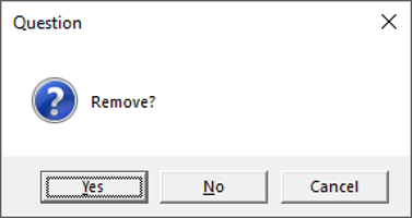
target.colname = "KCAL", min = 650, max = 5700)This function will print out rows that fall outside the specified min-max range, and a dialogue box will appear outside the R Studio (shown below), asking whether to remove them. You should make sure to review these records carefully to double-check if the removal is warranted. It is possible to have a valid record that could meet the threshold for removal. Only you will know if you can trust the record when working with real data.
If you find potential outlier(s) here, click “No”, and view those total(s) with their other nutrient intake information by running the following;
KCAL_outliers <- subset(QCtotals, KCAL < 650 | KCAL > 5700) Sort the rows by KCAL and show only the specified variables.
KCAL_outliers[order(KCAL_outliers$KCAL, decreasing = T),
              c('SEQN', 'KCAL', 'GRMS', 'PROT', 'TFAT', 'CARB')]
Click to expand output
##       SEQN   KCAL      GRMS    PROT    TFAT    CARB
## 101  83966 8491.5  6612.205 335.830 410.320 884.400
## 2299 88940 7599.5  6931.510 262.960 385.590 782.480
## 384  84596 6080.0  8918.225 218.135 221.240 541.610
## 27   83790 6063.0 13353.210 181.210 197.205 908.415
## 3786 92345 5935.0 11337.440 268.665 190.195 680.740
## 1651 87422 5867.5  4568.280 161.715 263.075 746.130
## 1075 86100 5814.5  6231.715 211.370 287.185 541.640
## 187  84142 5781.0  4759.985 226.360 274.255 618.230
## 2641 89721  622.5   693.175  18.525  16.100 102.970
## 135  84030  604.0  1117.965  30.410  19.190  76.670
## 2670 89788  571.5  1128.650  17.845   8.095 111.245
## 79   83919  526.5  1564.250  15.820  29.545  49.240
## 4284 93441  512.0   975.250  25.215  16.265  66.575
## 1905 88064  496.0  4741.915  11.470  19.845  67.985
## 2892 90318  485.5  1840.470  27.125  23.185  41.555
## 903  85743  470.0   256.670  15.490  19.360  58.485
## 109  83987  442.0   737.375  11.170  15.975  65.050
## 3583 91849  439.0   586.075  14.855  14.055  63.875
If you think they are true outlier(s), then run the QCOutliers command for KCAL again, and click “Yes” to remove the outlier. Here for this tutorial, we will remove this individual.
QCOutliers(input.data = QCtotals,
           target.colname = "KCAL", min = 650, max = 5700)
## There are 18 observations with < 650 or > 5700 .
## Remove? (Yes/no/cancel)
## Outlier rows were removed; the cleaned data is saved as an object called "QCtotals".
## 2078 rows remained.Continue the QC process with other variables.
Flag if PROT is <25 or >240 → ask remove or not→ if yes, remove those rows.
QCOutliers(input.data = QCtotals,
           target.colname = "PROT", min = 25, max = 240)
## There are 12 observations with < 25 or > 240 .
## Remove? (Yes/no/cancel)
## Outlier rows were removed; the cleaned data is saved as an object called "QCtotals".
## 2066 rows remained.Flag if TFAT is <25 or >230 → ask remove or not → if yes, remove those rows.
QCOutliers(input.data = QCtotals,
           target.colname = "TFAT", min = 25, max = 230)
## There are 38 observations with < 25 or > 230 .
## Remove? (Yes/no/cancel)
## Outlier rows were removed; the cleaned data is saved as an object called "QCtotals".
## 2028 rows remained.Flag if VC (Vitamin C) is <5 or >400 → ask remove or not → if yes, remove those rows.
QCOutliers(input.data = QCtotals,
           target.colname = "VC", min = 5, max = 400)
## There are 64 observations with < 5 or > 400 .
## Remove? (Yes/no/cancel)
## Outlier rows were removed; the cleaned data is saved as an object called "QCtotals".
## 1964 rows remained.Name the males totals after QC.
QCed_M <- QCtotalsQC for females
Define your female totals dataset to be used as input.
QCtotals <- meantotal12d_demo_F Flag if KCAL is <600 or >4400 → ask remove or not → if yes, remove those rows.
QCOutliers(input.data = QCtotals, target.colname = "KCAL", min = 600, max = 4400)## There are 27 observations with < 600 or > 4400 .
## Remove? (Yes/no/cancel)
## Outlier rows were removed; the cleaned data is saved as an object called "QCtotals".
## 2278 rows remained.Flag if PROT is <10 or >180 → ask remove or not → if yes, remove those rows
QCOutliers(input.data = QCtotals, target.colname = "PROT", min = 10, max = 180)## There are 5 observations with < 10 or > 180 .
## Remove? (Yes/no/cancel)
## Outlier rows were removed; the cleaned data is saved as an object called "QCtotals".
## 2273 rows remained.Flag if TFAT is <15 or >185 → ask remove or not → if yes, remove those rows
QCOutliers(input.data = QCtotals, target.colname = "TFAT", min = 15, max = 185)## There are 20 observations with < 15 or > 185 .
## Remove? (Yes/no/cancel)
## Outlier rows were removed; the cleaned data is saved as an object called "QCtotals".
## 2253 rows remained.Flag if VC (Vitamin C) is <5 or >350 → ask remove or not → if yes, remove those rows.
QCOutliers(input.data = QCtotals, target.colname = "VC", min = 5, max = 350)## There are 53 observations with < 5 or > 350 .
## Remove? (Yes/no/cancel)
## Outlier rows were removed; the cleaned data is saved as an object called "QCtotals".
## 2200 rows remained.Name the females totals after QC.
QCed_F <- QCtotalsCombine the rows of M and F.
QCtotals_MF <- rbind(QCed_M, QCed_F)Now, you have prepared formatted and QC-ed food items, totals for each day, and mean totals across two days for each participant.
Adjust totals and items after QC
Remove the QC-ed individual(s) from the totals each day
In the previous section, we have removed individual(s) that did not pass the QC from mean total data. We will remove those individual(s) from the totals (calculated in B-2, before taking means of days), so that we will have the same individuals in QC-ed mean_total and total for each day.
Among the individuals in total12d_demo, select only those in QCtotals_MF.
total12d_demo_QCed <- total12d_demo[total12d_demo$SEQN %in% QCtotals_MF$SEQN, ]Save as a .txt file. This will be the total for each of the “QC-ed” individuals for each day, if you would like to perform clustering analyses with Day 1 and Day 2 separately.
write.table(total12d_demo_QCed, "Total_D12_FC_QC_eachday_demo_QCed.txt", sep="\t", quote=F, row.names=F)Similarly, remove the QC-ed individual(s) from the food items to be consistent with the QC-ed averaged totals
Among the individuals in food12f_demo (generated in Procedure A), select only those in QCtotals_MF.
food12f_demo_QCed <- food12f_demo[ food12f_demo$SEQN %in% QCtotals_MF$SEQN, ]Save as a .txt file. This will be the items for each of the “QC-ed” individuals for each day, to be used for ordination etc.
write.table(food12f_demo_QCed, "Food_D12_FC_QC_demo_QCed.txt", sep="\t", quote=F, row.names=F)Come back to the main directory before you start running another script.
setwd(main_wd)