Data overview of GLU-index
Introduction
We added GLU_index to the QC-ed totals in the previous script. In this script, we will analyze some of the body measurements and KCAL intake by GLU_index groups using the QC-ed totals data. These examples are not intended to be a complete guide to analysis, but rather to give you some ideas for how to explore this data.
Load functions and packages
Name the path to DietR directory where input files are pulled.
main_wd <- "~/GitHub/DietR"Load the necessary functions.
source("lib/specify_data_dir.R")
source("lib/ggplot2themes.R")
You can come back to the main directory by:
setwd(main_wd)Specify the directory where the data is.
SpecifyDataDirectory(directory.name= "eg_data/NHANES/Laboratory_data/")Load the mean totals and check the variables’ distributions by GLU_index levels
Load the data of those to be used in the diabetic status analysis.
glu_2 <- read.table( file="QCtotal_d_ga_body_meta_glu_comp_2.txt", sep= "\t", header= T )Make GLU_index as a factor for plotting.
glu_2$GLU_index <- factor(glu_2$GLU_index, levels = c("Normal", "Prediabetic", "Diabetic"))BMI frequency of each group
The columnname for BMI is BMXBMI.
Check the summary data - this will also show the number of missing data if any.
summary(glu_2$BMXBMI)## Min. 1st Qu. Median Mean 3rd Qu. Max. NA's
## 16.00 24.10 28.20 29.21 33.00 63.60 1313 are missing BMI and has NA’s. You can also see that by counting the number of NAs in specified rows.
colSums(is.na(glu_2[, c("SEQN", "BMXBMI")]))## SEQN BMXBMI
## 0 13Create a density plot of BMI by GLU_index type.
BMIfreq <- ggplot(data=glu_2, aes(x=BMXBMI, group=GLU_index, fill=GLU_index)) +
  geom_density(adjust=1.5, alpha=.4) + space_axes + no_grid +
  scale_fill_manual(values= c("steelblue3", "yellow", "hotpink") ) +
  labs(x="BMI", y="Density")
Print out the chart. > If there are missing data, it will give a Warning message: > “Removed 13 rows containing non-finite values (stat_density).”
BMIfreq## Warning: Removed 13 rows containing non-finite values (`stat_density()`).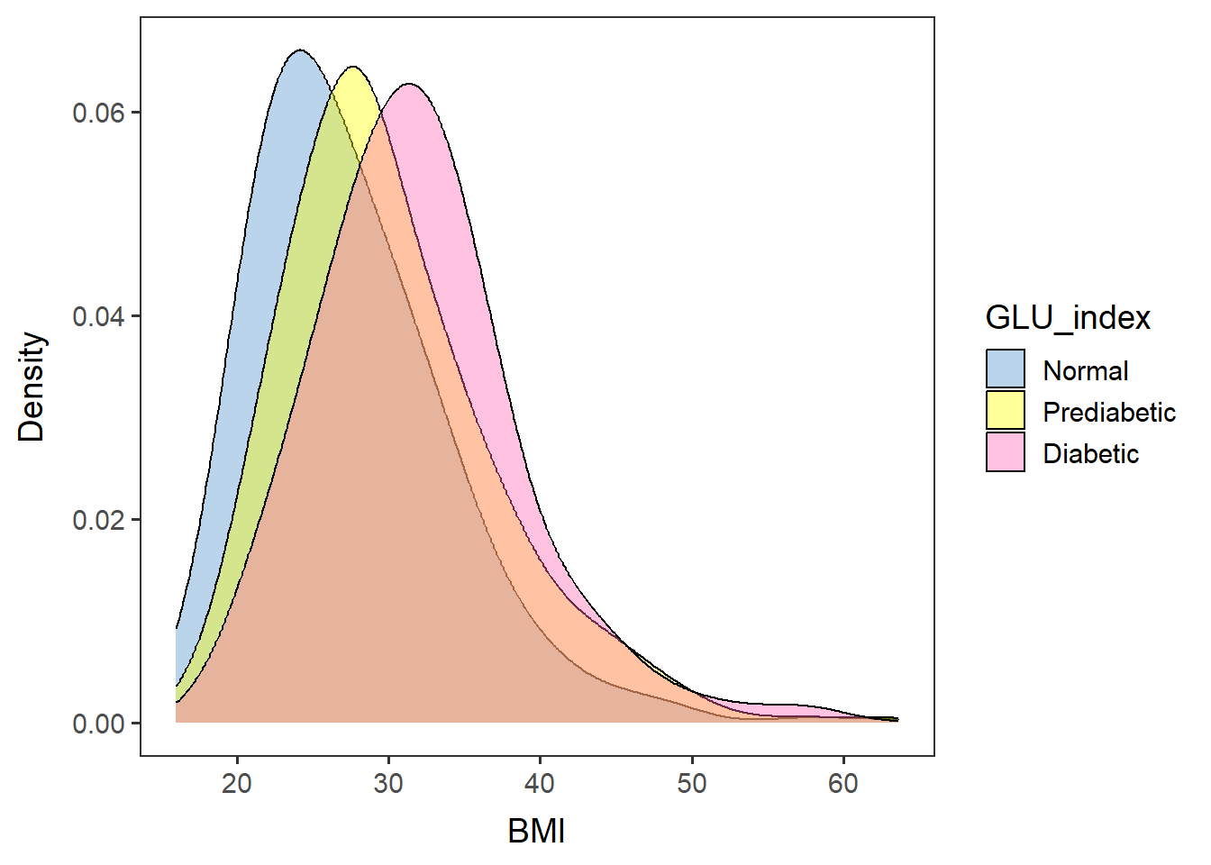
Save the chart as .pdf. It is helpful to make note of the number of datapoints: n = 1610 - 13 missing = 1597.
ggsave("QCtotal_d_ga_body_meta_glu_comp_2_n1597_BMI_by_GLU_index.pdf",
       BMIfreq, device="pdf", width=5.3, height=4.5)
## Warning: Removed 13 rows containing non-finite values (`stat_density()`).The diabetic population seems to have higher BMI than the prediabetic, and the lowest BMI was the normal population.
Bodyweight frequency of each group
The columnname for bodyweight is BMXWT.
Check the summary data - this will show the number of missing data if any.
summary(glu_2$BMXWT)## Min. 1st Qu. Median Mean 3rd Qu. Max. NA's
## 36.00 65.80 78.40 81.35 92.65 198.90 1111 are missing body weight and has NA’s.
Show histogram of body weight.
hist(glu_2$BMXWT)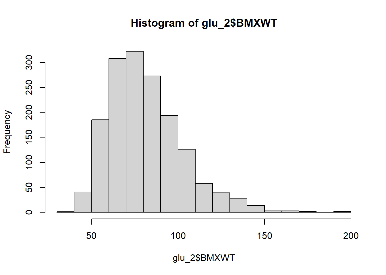
Create a density plot of body weight by GLU_index type.
weightfreq <- ggplot(data=glu_2, aes(x=BMXWT, group=GLU_index, fill=GLU_index)) +
  geom_density(adjust=1.5, alpha=.4) + space_axes + no_grid +
  scale_fill_manual(values= c("steelblue3", "yellow", "hotpink")) +
labs(x="Body weight (kg)", y="Density")weightfreq## Warning: Removed 11 rows containing non-finite values (`stat_density()`).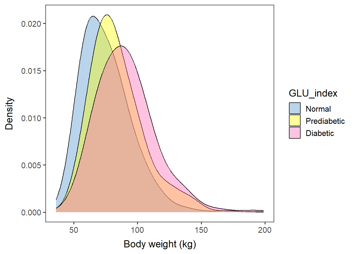
Save the chart as .pdf. n = 1610 - 11 missing = 1599.
ggsave("QCtotal_d_ga_body_meta_glu_comp_2_n1599_weight_by_GLU_index.pdf",
       weightfreq, device="pdf", width=5.3, height=4.5)
## Warning: Removed 11 rows containing non-finite values (`stat_density()`).KCAL frequency of each group
Check the summary data - this will show the number of missing data if any.
summary(glu_2$KCAL)## Min. 1st Qu. Median Mean 3rd Qu. Max.
## 604.5 1518.0 1933.5 2022.3 2444.9 5136.0There is no missing data for KCAL.
Create a line chart of the KCAL frequency of each group.
KCALfreq <- ggplot(data=glu_2, aes(x=KCAL, group=GLU_index, color=GLU_index)) +
  geom_density(adjust=1.5, alpha=.4, linewidth=1.2, linetype="longdash") + space_axes + no_grid +
  scale_color_manual(values= c("steelblue3", "gold3", "hotpink") ) +
  labs(x="KCAL", y="Density") +
  scale_y_continuous(labels = function(x) format(x, scientific = FALSE))
KCALfreq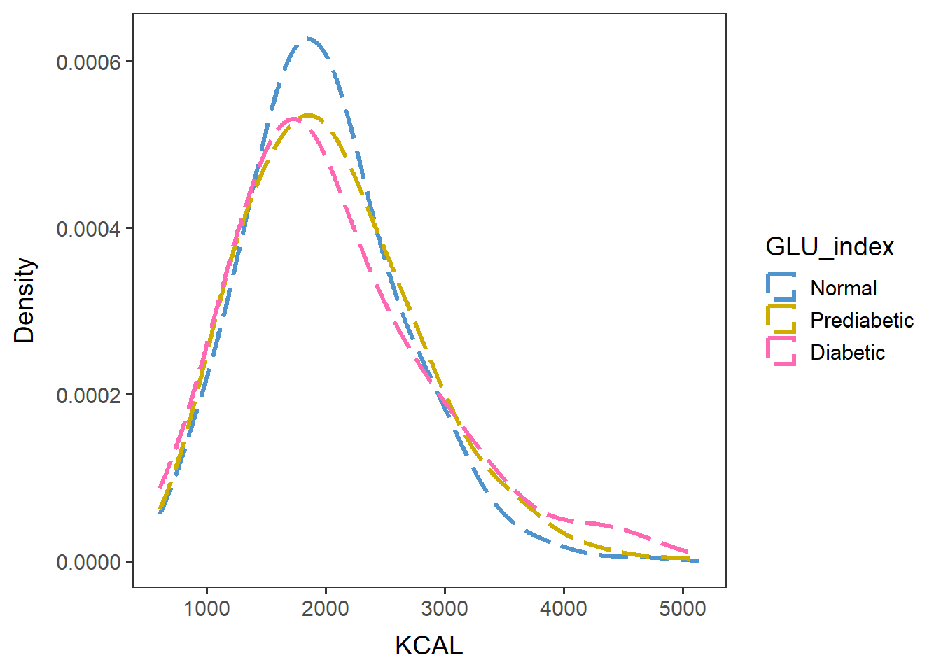
Save the chart as .pdf.
ggsave("QCtotal_d_ga_body_meta_glu_comp_2_n1610_KCAL_by_GLU_index_line.pdf",
       KCALfreq, device="pdf", width=5.3, height=4.5)
Come back to the main directory before you start running another script.
setwd(main_wd)