Visualize ordination
Introduction
There may be cases where you want to highlight specific users in the biplot because they have distinct metadata etc. Individuals can be highlighted with a thicker outline if desired. This can be done by loading the saved ordination results - Axis values and metadata combined, and the proportion of variance explained.
Load functions and packages
Name the path to DietR directory where input files are pulled.
main_wd <- "~/GitHub/DietR"Load necessary packages.
library(ggplot2)Load the necessary functions.
source("lib/specify_data_dir.R")
source("lib/ggplot2themes.R")
Load the distinct 100 colors for use.
distinct100colors <- readRDS("lib/distinct100colors.rda")You can come back to the main directory by:
setwd(main_wd)Specify the directory where the data is.
SpecifyDataDirectory(directory.name = "eg_data/NHANES")Load ordination results
Change to the folder called “Ordination”.
SpecifyDataDirectory(directory.name = "eg_data/NHANES/Laboratory_data/Ordination/")Read in the metadata and users’ Axis values.
loaded_glu_w <- read.table("Food_D12_FC_QC_demo_QCed_males60to79_3Lv_ord_WEIGHTED_meta_users.txt",
                           sep="\t", header=T)
Convert the GLU_index as a factor to plot it in order.
loaded_glu_w$GLU_index <- factor(loaded_glu_w$GLU_index, levels= c("Normal", "Prediabetic", "Diabetic"))Load the eigenvalues as a vector.
eigen_loaded <- read.table("Food_D12_FC_QC_demo_QCed_males60to79_3Lv_ord_WEIGHTED_eigen.txt", header=T)Make a vector that contains the variance explained.
eigen_loaded_vec <- eigen_loaded[, 2]Create a folder called “Viz_Ordination” to save the plots to be produced here.
Highlight certain sample(s) - e.g. participants 83755 and 83820
Subset datapoint(s) that you would like to highlight.
select_point <- subset(loaded_glu_w, SEQN=="83755" | SEQN=="83820" ) Plot participants in different colors, then plot the selected participants (SEQNs) above with a thicker outline.
highlighted <- ggplot() +

  # Plot all the datapoints first.
  geom_point(loaded_glu_w, shape=21, size=3, alpha=1, colour="black",
             mapping=aes(x=Axis.1, y=Axis.2, fill=GLU_index)) +
  scale_fill_manual(values = c("steelblue3", "yellow", "hotpink")) +
  xlab( paste("Axis.1 (", paste(round(eigen_loaded_vec[1]*100, 1)), "%)", sep="") ) +
  ylab( paste("Axis.2 (", paste(round(eigen_loaded_vec[2]*100, 1)), "%)", sep="") ) +
  no_grid + space_axes + theme(aspect.ratio = 1) +

  # Add thicker outlined datapoints of selected individuals.
  geom_point(select_point, shape=21, size=3, alpha=1, stroke=2, color="black",
             mapping=aes(x=Axis.1, y=Axis.2, fill= GLU_index), show.legend=F) +

  # Add a caption to explain the highlighted datapoint(s).
  labs(caption="SEQN 83755 and 83820 are highlighted with a thick outline.") +
  theme(plot.caption =  element_text(hjust=1, face="italic"))
highlighted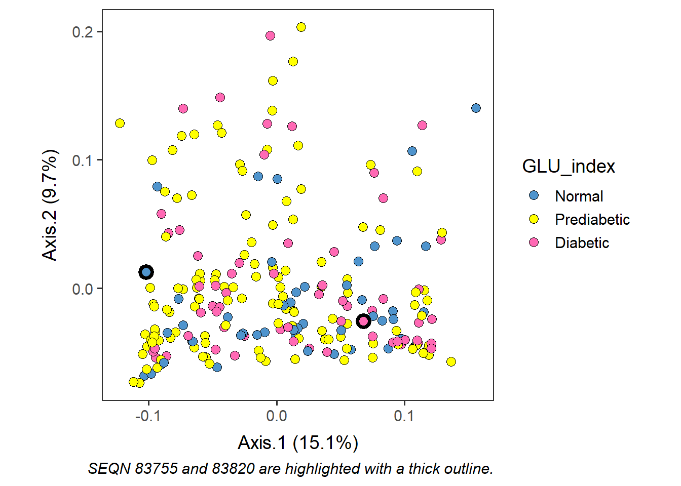
ggsave("Viz_Ordination/Food_D12_FC_QC_demo_QCed_males60to79_3Lv_ord_WEIGHTED_Axis12_highlighted.pdf",
       highlighted, device="pdf", width=7, height=5.5, unit="in", dpi=300)
Come back to the main directory.
setwd(main_wd)