Visualize foodtrees
Introduction
Here, we will use the ggtree package to plot foodtrees generated in the previous script.
Load functions and packages
Name the path to DietR directory where input files are pulled.
main_wd <- "~/GitHub/DietR"If you have not downloaded and installed the ggtree package yet, you can do so by first installing BiocManager (if you have not done so):
if (!require("BiocManager", quietly = TRUE))install.packages("BiocManager")Then, use BiocManager to install the “ggtree” package.
BiocManager::install("ggtree")Load necessary packages.
library(ggtree)Load the necessary functions.
source("lib/specify_data_dir.R")
source("lib/viz_food_tree.R")
You can come back to the main directory by:
setwd(main_wd)Visualize your food tree
Specify where your data is.
SpecifyDataDirectory("eg_data/NHANES/Laboratory_data/Foodtree")Load your tree object.
tree <- read.tree("Food_D12_FC_QC_demo_QCed_males60to79_3Lv.nwk") It is OK to see an error that says:
Found more than one class “phylo” in cache; using the first, from namespace ‘phyloseq’
Also defined by ‘tidytree’
Prepare the tree data for visualization.
PrepFoodTreePlots(input.tree = tree)Create a color-coded and annotated food tree with 9 L1 levels.
It is OK to see some warning messages that say:
Coordinate system already present. Adding new coordinate system, which will replace the existing one.
Scale for ‘y’ is already present. Adding another scale for ‘y’, which will replace the existing scale.
VizFoodTree(input.tree=tree, layout="circular") ## Coordinate system already present. Adding new coordinate system, which will
## replace the existing one.
## Scale for y is already present.
## Adding another scale for y, which will replace the existing scale.
## Scale for y is already present.
## Adding another scale for y, which will replace the existing scale.
## Coordinate system already present. Adding new coordinate system, which will
## replace the existing one.Take a look at the tree.
annotated_tree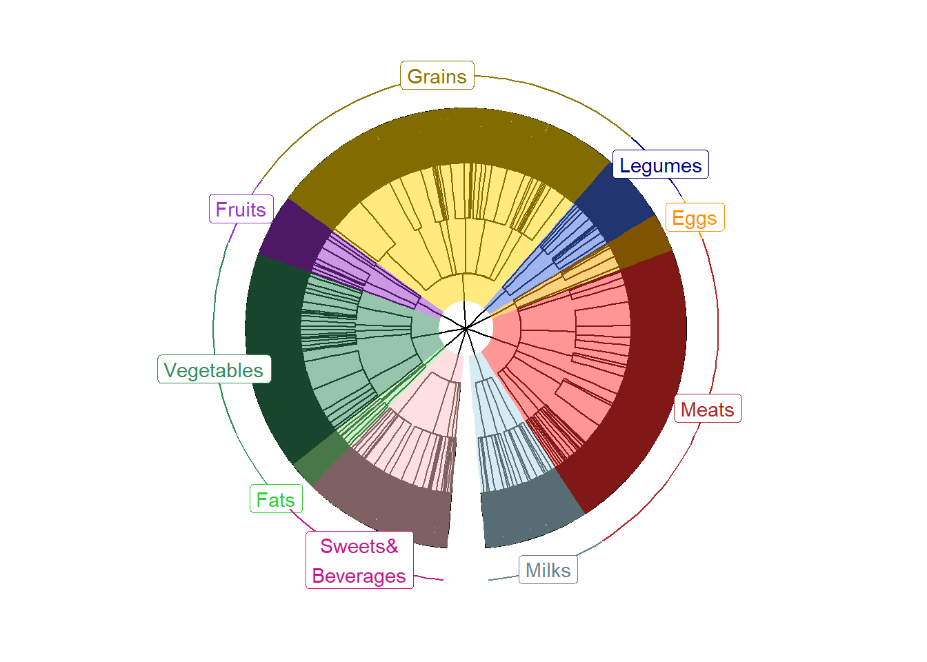
Save.
ggsave("Food_D12_FC_QC_demo_QCed_males60to79_3Lv_viz.pdf", annotated_tree,
       device="pdf", width=5.2, height=5)
You can also visualize trees of different levels; Lv2, Lv3, etc., which corresponds to the classification depth of each food item in the dataset. For example, Lv3 contains L1, L2, and L3 categories of food; whereas Lv4 contains L1, L2, L3, and L4 categories. Thus, as the level goes deeper, the more internal nodes there will be in the foodtree.
Come back to the main directory.
setwd(main_wd)